INSIDE A TYPICAL SPICE FILE
The heart of your SPICE file is the netlist, which is simply a list of components and the nets (or nodes) that connect them together. As an example, we'll create a netlist for a simple low-pass RC filter. Just draw the schematic, then assign names for the resistor, capacitor, voltage source (R1, C1, VS) and node numbers (1 and 2). Ground is the only exception whose node is always numbered 0.
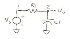
Then generate a text file like the one below.
LPFILTER.CIR - SIMPLE RC LOW-PASS FILTER
*
VS	1	0	AC 1 SIN(0VOFF 1VPEAK 2KHZ)
*
R1	1	2	1K
C1	2	0	0.032UF
*
* ANALYSIS
.AC 	DEC 	5 10 10MEG
*.TRAN 	5US  500US
*
* VIEW RESULTS
.PROBE
.END
COMPONENTS
As you can see, much of the netlist is intuitively obvious: name a component, designate the nodes where it's connected, and give it a value. For example,
RS 1 2 1000
describes a 1000 ohm resistor connected between nodes 1 and 2. Just follow a few rules - all resistors names begin with R, capacitors with C, voltage sources with V, etc. For more information go to SPICE Command Summary.
VOLTAGE SOURCE
SPICE has many voltage sources available: SINE, PULSE, AC, DC, etc. For this example, the voltage source statement has two functions.
VS 1 0 AC 1 SIN(0V 0.2V 10kHz)
First, it creates an AC signal source between nodes 1 and 0 for AC (frequency) Analysis. Second, it also generates a sinewave source SIN for the Transient (time) Analysis. This sine wave has a DC offset of 0 V, a peak amplitude of 0.2 V and a frequency of 10 kHz.
AC AND TRANSIENT ANALYSIS
SPICE is capable of performing both AC (frequency) Analysis and Transient (time) Analysis. SPICE also performs a number of other analyses like DC, Sensitivity, Noise and Distortion. The command
.AC DEC 5 10 10MEG
tells SPICE to run an AC Analysis at 5 points per DECade in the frequency range from 10 Hz to 10 MHz. The command
.TRAN 0.001MS 0.2MS
requests a Transient (time) Analysis TRAN for a duration of 0.2 ms and prints out the results
at 0.001 mS intervals.
NOTE: Some SPICE versions allow either .TRAN or .AC but NOT both!
Simply comment out the undesired analyis by placing a "*" at the beginning
of the statement.
What analysis results do you want to see? Most SPICE versions today automatically open a separate plot window after running a simulation. Through pull-down menus typically named Add Plot or Add Trace, you can enter variables like V(2) or I(R1) to be plotted.
Some viewers list all of the variables and you just click on the ones you want to see. As a bonus many plotting windows let you enter calculations like V(2)*I(VS) or V(2)-V(1). The more sophisticated versions go a step further by providing operations on variables like AVG( V(2) ) or RMS( V(2)*I(VS) ).
You can display the magnitude, real part, imaginary, part, phase, etc of the variables for the AC Analysis. Just add the appropriate suffix as follows:
| Voltage | Current | Variable |
| V( ) | I( ) | (no suffix) Magnitude |
| VM( ) | IM( ) | Magnitude |
| VP( ) | IP( ) | Phase |
| VR( ) | IR( ) | Real Part |
| VI( ) | II( ) | Imaginary Part |
Some versions of SPICE also print the results to a text file named filename.OUT. The PRINT command places the numerical results in a table.
.PRINT AC VM(2)
.PRINT TRAN V(1) V(2)
The statements above prints the voltage magnitude at node 2 for the AC Analysis and the voltages at nodes 1 and 2 for the Time Analysis.
The PLOT command creates a line-printer like graph of the data.
.PLOT TRAN V(1) V(2)
.PLOT AC VM(2)
Both results are generated in a text file named LPFILTER.OUT
You can add a comment or ignore any statements by placing a “*” at the beginning of the line. This is a great way to label circuit sections, include some simple notes in the file, or remove a component.
WHY USE SUBCIRCUITS?
You can think of a subcircuit as being similar to a subroutine in software programming. Just as subroutines uses the single definition of code many times over, a subcircuit uses the definition of a circuit many times over. This saves the tedium of creating multiple blocks of a circuit used in many places. A model of an op amp is good example of using a subcircuit. One model can be used in multiple amplifiers of your circuit. If you need to change all of the op amps, just change the single definition of the subcircuit.The subcircuit is defined by the statements
.SUBCKT < sub name> <node A> <node B> ...
Subcircuit definition.
.ENDS
The node numbers and component names in the definition will be separate from those in the main circuit. The only exception is node 0, the global ground reference. To place your subcircuit into the main circuit use the statements
XCirName <node 1> <node 2> ... <definition name>
When the simulation is run, a subcircuit is created with its <node A> connected to <node 1> of the main circuit and so on.
SUBCIRCUIT EXAMPLE
Here’s a quick example to show how a subcircuit called “OPAMP1” is used for both devices XOP1 and XOP2 in a cascaded amplifier circuit. We’ve labeled the subcircuit node numbers in parentheses for clarity.
Here’s a SPICE subcircuit schematic for the guts of an op amp.
The complete netlist of the circuit appears below.
AMP2.CIR – CASCADED OPAMPS
*
VS	1	0	AC	1	SIN(0 1 10KHZ)
*
R1	1	2	5K
R2	2	3	10K
XOP1	0 2	3	OPAMP1
R3	4	0	10K
R4	4	5	10K
XOP2	3 4	5	OPAMP1
*
* SINGLE-POLE OPERATIONAL AMPLIFIER MACRO-MODEL
* connections:      non-inverting input
*                   |   inverting input
*                   |   |   output
*                   |   |   |
.SUBCKT OPAMP1      1   2   6
* INPUT IMPEDANCE
RIN     1          2          10MEG
* DC GAIN (100K) AND POLE 1 (100HZ)
EP1	3 0	1 2	100K
RP1	3	4	1K
CP1	4	0	1.5915UF
* OUTPUT BUFFER AND RESISTANCE
EOUT	5 0	4 0	1
ROUT	5	6	10
.ENDS
*
* ANALYSIS
.TRAN	0.01MS  0.2MS
* VIEW RESULTS
.PLOT TRAN V(1) V(5)
.END
The subcircuit is defined between the statements
.SUBCKT OPAMP1 1 2 6 and .ENDS
The subcircuit OPAMP1 gets inserted into two places of the main circuit by the statements
XOP1 0 2 3 OPAMP1
XOP2 3 4 5 OPAMP1
For XOP1, the subcircuit nodes (1), (2) and
(6)
connect to main circuit
nodes 0, 2 and 3.
Likewise for XOP2 the subcircuit nodes
(1), (2) and (6)
connect to main circuit nodes 3, 4 and 5.
You can try a different op amp
device in both stages by simply changing the OPAMP1 subcircuit definition.
The default units for SPICE are volts, amps, ohms, farads, henries, watts etc. You can specify values in decimal form, 0.0056, or exponential form, 5.6e-3. SPICE also recognizes the following abbreviations:
|
F |
E-15 |
femto |
|
P |
E-12 |
pico |
|
N |
E-9 |
nano |
|
U |
E-6 |
micro |
|
M |
E-3 |
milli |
|
|
|
|
|
K |
E+3 |
kilo |
| MEG | E+6 | mega |
| G | E+9 | giga |
| T | E+12 | tera |
For clarity you can add letters to the abbreviation as in 1U or 1UFARADS and both are read as the value 1e-6.. SPICE processes the first letter after the number and ignores the rest.
Having a SPICE reference on your shelf may come in handy as your circuit adventures continue. Check out the following books on SPICE.
SPICE: A Guide to Circuit Simulation and Analysis Using PSpice, Paul Tuinenga, 3rd Edition, Prentice-Hall, 1995, ISBN 0-13-158775-7.
The Spice Book, Andrei Vladimirescu, John Wiley & Sons, Inc.,
1994, ISBN 0-471-60926-9.PSpice and Circuit Analysis, John Keown, Third Edition, Merrill (Macmillan Publishing Company), 1997, ISBN 0-13-235458-6.
© 2002-2023 eCircuit Center