Op Amp Control System - Part 1
CIRCUIT

OP_CONTROL1.CIR Download the SPICE file
This classic control topology lies at the heart of many types of control systems: temperature, speed, position, etc. I've also seen them control voltages and currents of power supplies in early HP designs and in the latest test equipment. The beauty of this circuit is it's simplicity and wide application. How does it work and how can you apply it to your application? Part 1 walks through the basic circuit and shows you a simple approach to understanding and applying it. In Part 2, we'll cast the elements into control system blocks. Then we'll walk though some loop analysis (open and closed) to better understand and optimize it for a quick and accurate response.
AUTOMATIC CONTROL
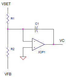
There's only a few components to this circuit: an op amp, two
resistors and a cap. The rest is basic control stuff. As far as the op
amp circuit goes, it sees only two signals, the set point VSET and the
feedback voltage from the sensor VFB.

Operation is simple: adjust the control output VC to make VFB equal and
opposite VSET. How is this leveraged to achieve motion control, for example?
Suppose you have a tachometer that generates
1V / 100 RPM. To get the
motor spinning at 1,000 RPM, set VSET = -10V. The circuit automatically
adjusts VC (the signal driving the amp / motor) until VFB =
+10V. This +10V level from the tachometer represents +10V x 100 RPM / V =
1,000 RPM.
HOW IT WORKS
The
circuit combines two basic circuits: a summing amp and an inverting integrator. The
summing portion works by the op amp holding its negative input to ground and
summing the currents that flow into R1 and R2.

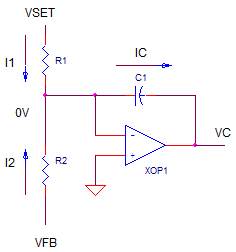
VSET and VFB force two currents written simply as
I1 = VSET / R1
I2 = VFB / R2
How about the current in C1? According to Kirchoff currents law,
IC = I1 + I2
= VSET / R1 + VFB / R2
IC gets integrated on C1 forcing the output VC to move positive or negative. The prime directive of this circuit is to bring VFB to be equal and opposite of VSET. In this condition, IC = 0 and the output voltage VC does not change further..
Let's follow circuit operation (R1 = R2 = 10k, CI = 1000pF) from the time you give the command to move until target speed is reached. To get a positive output, VSET will be set negative (-10V) such that VFB will achieve an equal and opposite value (+10V). Let's look at three instances.
| Speed | Set Point and Feedback | What Happens | |
| Zero Speed | Change
VSET from 0V to -10V VFB = 0V (Speed = 0 RPM). |
IC = I1 + I2 = -10/10k + 0V/10k =
-10mA All of I1 dumps onto CI! VC rises rapidly as CI integrates -10mA. Motor begins rotating, VFB begins to rise. |
|
| Half Speed |
VSET = -10V VFB = +5V (Speed = 500 RPM) |
IC = I1 + I2 = -10/10k + 5V/10k =
-5mA Only half the original l0mA is integrated onto CI. VC rises more slowly as CI integrates -5mA. VFB continues to rise. |
|
| Full Speed | VSET =
-10V VFB = +10V (Speed = 1000 RPM). |
IC = I1 + I2 = -10/10k + 10V/10k =
0mA No current into C1. VC holds steady, 0mA into CI causes no voltage change. VFB holds at 10V. Target speed has been achieved! |
Why Bother? If the power amp and motor produce an output of 100 RPM / V, why not just drive the power amp's input with, say 10V, and get the desired 1,000 RPM? Forget the added complexity and cost of the control system. Although this sounds straightforward, in reality the power amp and motor typically have large tolerances. How can you achieve 1% speed accuracy with a motor with 5% speed tolerance?
To make matters worse, the motor speed specification is given with no load on the motor. Connect a load to the motor shaft to a gear system to lift or move a mechanism and watch the motor speed drop significantly due to friction losses. To save the day, the control system automatically adjusts the drive higher or lower to maintain the desired speed.
SPICE SYSTEM MODEL

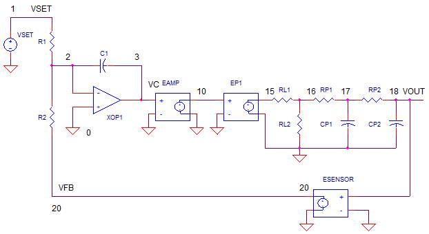
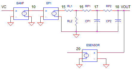
POWER AMP EAMP represents the power amp. Why do you need one? The power amp delivers the current needed. U1 can only provide small output current (1-40 mA), a small fraction of Amps it can take to move a motor or drive a heater. The amp also has a hard limit of +/-15V modeling an amplifier hitting the power supply rails.
PROCESS EP1 represents a very simplified model of a process to be controlled like motor velocity or heater temperature. The gain of 100 could represent an output transfer function of 100 RPM / V or 100 ° C / V.
LOSSES AND DELAY The system losses are modeled by a simple resistor divider RL1 and RL2. The time delay caused by the motor's inertia or heater's thermal mass are modeled by a simple low-pass filter RP1, CP1, RP2 and CP2.
SENSOR The final element in the chain is the feedback element (tachometer or thermocouple for example.) Although V(18) simulates in volts, we know it really represents output variables like speed in RPM or temperature in °C. For our motor simulation, we'll assume units of RPM. It creates an output of 1V per 100 RPM.
RESPONSE TIME
How can control how fast the control loop responds to VSET? R1, R2,
and C1 set the response time. For a steady current through C1 over time
∆T, the output VC changes by
∆VC = ( IC ·
∆T) / C1
So, the smaller you make C1, the faster the VC changes. Like wise, the
smaller you make R1 and R2 (the bigger IC gets), the faster VC responds.
Danger Ahead! You may be tempted to make R1, R2, C1 as small possible to allow the control loop to respond at blazing speeds. Not so fast! There's potential danger when the control response time is shorter than the time delay of the motor or heater. You'll see below that the results are not so pretty when the system runs out of control.
THE BASIC TEST
Let's take this motor out for a spin. Then we'll change the tolerance and
apply losses to see if the control system can hold its promise of holding the
speed steady under varying conditions. Voltage source VS drives the op amp's
input with -10V step input. The target speed is 10V * 100 RPM/V = 1000
RPM.
CIRCUIT INSIGHT Run a Transient Analysis (Time domain) using the .TRAN statement. Plot the the set point V(1) and the feedback (tachometer) output V(20). Does V(20) swing equal and opposite of V(1)? Open another plot window and plot the actual speed at V(18) where Volts represents RPM. Does the motor speed reach its target of 1000? Open another window and plot the control voltage VC at V(3) and amplifier output at V(10).
TOLERANCES Suppose the motor manufacturer sent you motor with a 5% tolerance - the motor spins at only 95RPM when you apply a volt to an unloaded motor. To model this, change the gain of EP1 from 100 to 95 times V(10). Rerun the simulation. Did speed at V(18) reach it's target? Wicked! This is the power of control systems - compensating for component variations in the chain. Check out V(3). This voltage rose to about 5% over the ideal value of 10V to compensate for -5% performance of the motor.
LOSSES Another dose of reality in any control system is the losses in the system. Let's say you've connected the motor to a gear with a heavy load like a moving walkway at the airport. The friction losses amount a 10% drop in speed if no control system were present. You can model this by changing resistor values to RL1 = 10 and RL2 = 90 to achieve a 10% drop in speed constant. Rerun the simulation and check the speed at V(18).
ACCURACY Ultimately, the accuracy falls on four components: R1, R2, the op amp and the feedback element (the tachometer.) Change R1 or R2 by 5% and see what happens to the speed at V(18)! Likewise change the speed constant at ESENSE by some factor, say 10%. What happens to your accuracy? Finally, any errors induced by the op amp (input offset and bias currents - not modeled here) will cause errors at VFB and consequently at the output speed. The ultimate lesson here: if you need accuracy, spend money on precision parts for these four components!
THE ADVANCED TEST
TIME DELAY
Nothing responds instantly - motors (gears/loads) have inertia
to overcome. You can get a sense for the finite time delay by plotting V(16)
along with V(18). You can think of this as the lag between the applied
torque and the motor changing speed. You'll notice that this time delay
is relatively short compared to the overall control loop rise time - a
good thing for keeping the loop in control..
RESPONSE TIME Okay, let's play with the speed dial. Slow the loop down by making C1 larger by 2x. Rerun the simulation and check out the output V(18) and the feedback V(20) - a dramatic change! (You can achieve the same change by making R1 and R2 2x larger.)
Now speed things up by change C1 to 2x smaller than the original. Did the output respond faster? Don't stop there, keep reducing C1 by 2x - see how fast you can make this loop go! What starts to happen? As the output rises faster, you'll see it start overshoot and ringing. Keep making C1 smaller and eventually the loop breaks into an ugly sustained oscillation. Why? Basically, the control loop is reacting too fast compared with the time delay of the system. It keeps over correcting trying to do it's job! Back off the speed a bit. Most designers find a compromise between a fast response and a little overshoot and ringing.
NEXT UP
This turned out to be a big topic for a small op amp circuit.
Congratulations on going the distance! The next topic in the works is the
sequel (Part 2) where we'll transform the circuit into classic control
blocks. Then, we'll turn on some loop analysis to give us the power to
predict it's speed and any oscillation condition.
The loop analysis tool will let you apply advanced design techniques like lead-lag filters to help speed up and stabilize troublesome loops that would oscillate otherwise.
SPICE FILE
Download the file
or copy this netlist into a text file with the *.cir
extention.
OP_CONTROL.CIR
*
* SET POINT
VS	1	0	AC 1	PWL(0US 0V   0.01US -10V)
*
* CLASSIC CONTROL AMPLIFIER
R1	1	2	100K
R2	20	2	100K
CI	2	3	1UF
XOP1	0 2     3       op_001
*
* POWER AMP WITH LIMIT
EAMP	10	0	VALUE = {  LIMIT( 1 * V(3), +15, -15 )  }
*
* PROCESS (MOTOR, HEATER, ETC)
EP1	15	0	VALUE = { 100 * V(10)  }
* LOSSES (FRICTION, HEAT LOSS, ETC.)
RL1	15	16	0.1
RL2	16	0	100
* DELAY (INERTIA, THERMAL MASS, ETC.)
RP1	16	17	100K
CP1	17	0	0.1UF
RP2	17	18	100K
CP2	18	0	0.1UF
*
* SENSOR (TACHOMETER, THERMISTOR, ETC.)
ESENSE	20	0	VALUE = { 1/100 * V(18)  }
*
*
 * BASIC OP AMP MODEL
* Device Pins     In+ In- Vout
.SUBCKT op_001    1   2   82
RIN   1   2   1e9
*   Aol=1000000, fu=1000000 Hz
G1   0    10  VALUE = { 1.0 * V(1,2)  }
R1   10   0   1e6
C1   10   0   1.59e-7
* OUTPUT STAGE
EOUT 80 0   10  0    1
ROUT 80     82    10
.ENDS
*
* ANALYSIS *************************************
.TRAN 	0.1MS  1000MS
*.AC 	DEC 	20 0.1 1000MEG
.PROBE
.END
2010 eCircuit Center