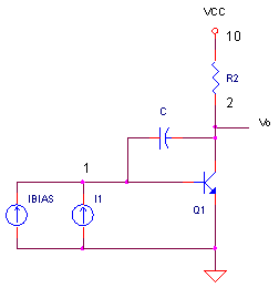
The Miller Integrator
CIRCUIT
MILLER_INTEGRATOR.CIR Download the SPICE file
At the heart of most audio amplifiers and op amps is a circuit that determines not only the bandwidth, but the slew rate too! This circuit is an integrator formed by strapping a capacitor across the input/output of a voltage gain stage. An integrator of this form is called the Miller Integrator as shown above. How does the circuit work? You can grind through the analysis to get an output equation. Problem is that it's messy and not very intuitive. Or, you can approximate its response by a simple integrator equation. This gives you a powerful tool for predicting your amplifier's performance. But where does the approximation succeed and fail? A quick simulation can show you.
SMALL SIGNAL MODEL
Here's a simplified version of the circuit above.
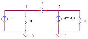
To use this circuit, we first need to describe how it works. Let's roll up our sleeves and solve for an equation relating the output (V2) to the input (I1). Calling on our basic training (and mine often needs refreshing), write the nodal equations for nodes 1 and 2, then solve for V2 / I1. Plowing through the equations you get
V2 (gm - s·C)·R1·R2
---- = ---------------------------------------
I1 s·C·(gm·R1·R2 + R1 + R2) + 1
Probably not the most intuitive equation you've seen! Maybe there's a simpler way to look at this.
IDEAL MILLER INTEGRATOR
A more idealized version of the Miller Integrator appears like one of these two circuits.
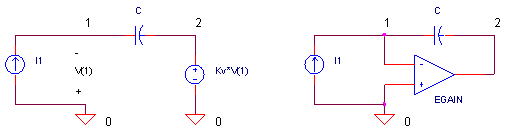
Basically, you've got an amplifier with large negative voltage gain and a capacitor strapped across the input / output. You can write the output as
V2 -Kv
---- = -------------
I1 1 + Kv·s·C
For large Kv, the gain simplifies to an equation that looks like an integrator (inverting).
V2 / I1 = -1 / (s · C)
Yes, this is a more friendly equation than the one above! Let's see if there's anything in common between the the frequency response of this simple integrator and the transistor version.
BANDWIDTH - SIDE BY SIDE
To pull it all together, let's check the AC response of three Miller Integrator circuits: 1) the transistor based circuit, 2) it's small-signal equivalent model and 3) the almost ideal integrator. For the small signal model, calculate the input resistance and transconductance (gm = ic / vin) with β = 100 and Ic = 1 mA.
R1 = β / (Ic / 26 mV) = 2.6 kΩ
gm = Ic / VT = Ic / 26 mV = 0.0385 A / V
The transistor gets biased at 1mA by setting Ibias = Ic / β = 1mA / 100 = 10 uA.
For the Ideal Integrator, it operates like its namesake by
setting its internal gain to a large value
like Kv = 1000.
CIRCUIT INSIGHT
Okay, let's see the Miller Integrators in action. Run an AC Analysis
and plot the outputs
V(2), V(22) and V(32). To get a better view, change the
y axis to a log scale. First question: how well does the small signal
model V(22) match the transistor response V(2)? Hopefully, these two plots should lay on top of one another. The second, and bigger question: how do
the responses compare to the ideal integrator V(32)? Add this trace and
compare the responses. What do you see. For mid frequencies, the three plots
lay directly on top of one another!
This is good news! Why? It means that we can approximate the rather complex behavior (and complex equations) of the transistor based Miller Integrator, by the simple response and equation of the Ideal Integrator. Although this applies only at mid-frequencies, it's usually sufficient to approximate the overall bandwidth and slew rate of circuits containing an Miller Integrator, like an audio or operational amplifier.
SLEW-RATE
The maximum slew-rate defines how fast (in Volts per us) that an output is capable of changing. In an audio amplifier, this is often determined by the Miller Integrator. How? The first stage typically has a maximum output current Imax when the input is over driven. This current gets fed to the Miller stage and integrated to produce a maximum voltage swing.
dV / dt = Imax / C
Let's inject a +/-1 mA current pulse into the Miller integrator with a 500 pF cap. What is the expected slew-rate? The equation predicts dV/dt = 1mA / 500pF = 2 V / us. Let's simulate the three Miller brothers and check their slew rates.
CIRCUIT INSIGHT Run a Transient Analysis and plot the outputs V(2)-10, V(22) and V(32). Notice, you've got to subtract 10V from the V(2). Why? The transistor collector is biased at 10V. So a simple subtraction removes the DC component. Two questions: 1) How well do the integrator outputs match and 2) Does the slew rate agree with our calculation?
HANDS-ON DESIGN Double or half the current pulse height. Rerun the simulation and see its effect on the integrator outputs. Do the same to the miller capacitance and check the output.
SPICE FILE
Download the file or copy this netlist into a text file with the *.cir extension.
MILLER_INTEGRATOR.CIR

* GAIN STAGE / MILLER EFFECT
I1  0 1  AC 1  PWL(0US 0A  0.01US 1MA  1US 1MA  1.01US -1MA  2US -1MA  2.01US 0MA)

IBIAS	0	1	DC	10UA
Q1	2 1	0	QNPN
C	1	2	500PF
R2	2	10	5K
VCC	10	0	DC	+15V


* SMALL-SIGNAL MODEL
I_1  0 21  AC 1  PWL(0US 0A  0.01US 1MA  1US 1MA  1.01US -1MA  2US -1MA  2.01US 0MA)
R_1	21	0	2600
C_	21	22	500PF
R_2	22	0	5000
GM1		22	0	21 0 0.038


* IDEAL INTEGRATOR
I__1  0 31  AC 1  PWL(0US 0A  0.01US 1MA  1US 1MA  1.01US -1MA  2US -1MA  2.01US 0MA)
RIN	31	0	1e12
C__	31	32	500PF
EGAIN		0 32	31 0 1000


.model	QNPN	NPN(BF=100)
*
* ANALYSIS
*
.TRAN	0.1US 3US
.AC DEC 5 10 1000MEG
.PROBE
.END
© 2008 eCircuit Center