Op Amp Model

About SPICE | SPICE Basics | Running SPICE | CIRCUIT COLLECTION | SPICE Commands | SPICE Demos and Downloads
About Us | Contact Us | Home | Search
 

Adding 2nd and 3rd Poles
to Improve Transient Response
 

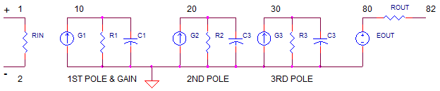
CIRCUIT

                                          OP_2ND_3RD_POLES.CIR   Download the SPICE file

It's relatively easy to create op amp SPICE models with a single pole (low-pass filter) in the gain stage. Testing the model by driving the input with a square wave shows an output with a nice smooth response. But wait! The data sheet typically shows a step response with some overshoot and ringing. How can you get your response to look more like the datasheet? You can move your model in the right direction by adding 2nd and 3rd poles at higher frequencies. But at what frequencies do we place these two low-pass filters? The answer lies in the datasheet and some simple trig.

OPEN LOOP FREQUENCY PLOT

One of the keys to getting the closed-loop overshoot and ringing right in the time domain, is getting the open-loop magnitude and phase right in the frequency domain. What does an open-loop frequency plot look like? The datasheet for a typical op amp will show something like this.

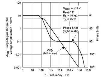
The plot shows the open-loop magnitude (left scale) and negative phase (right scale) versus frequency. A quick review about the plot. For a stable op amp (minimal overshoot an ringing), the phase should be greater than -180 deg at the frequency fu where the magnitude hits unity (0 dB).

What is the plot above telling us about this op amp?

1. We see the 1st pole around fp1=300 Hz. It adds -90 deg at f >> fp1.
    
2. MOST IMPORTANT: There's also a couple of additional poles adding about -22 deg at fu = 1 MHz. This brings the total phase to -90 – 22 = -112 deg. How much safety margin do we have before the phase hits -180 deg? We can calculate the phase margin as -112 - (-180) = 68 deg – this is considered a good margin that should produce a reasonable smooth response! A phase margin of 90 is even better. On the other hand, a phase margin of 0 deg and you've got yourself an oscillator!

ADDING NEGATIVE PHASE

So how can you make your SPICE model’s behavior include the additional negative phase like the plot above. I’ve seen models include a double pole at higher frequencies using simple RC filters. But where do you place the cutoff frequencies of these poles? The answer lies in the open-loop plot. Two simple steps can build you a better model.

1. Define the goal – I need to add θ_x amount negative phase at frequency fx.
2. Calculate the location of two identical poles fp2=fp3 to accomplish step 1.

Dusting off our basic circuits book, we rediscover that the phase θx of an RC low-pass filter at frequency fx, can be predicted by
                                  θx = tan-1 ( fx / fp)

where fp is the cutoff frequency of the pole. Now, solving for the fp we get,
                                  fp = -fx / tan (θx)

And once you have fp, all that needs calculating are the values of R and C.

Example: Looking at the graph, pick a convenient place to measure the added phase. Let's choose the point on the graph where -45 deg of phase shift occurs at f = 2 MHz. Yes, its not easy to read the exact values from the graph. But don't worry, we'll do some tweaking later.

1. Because we have two poles, each pole need only contribute half the phase.
                       θ = -45 / 2 = -22.5 deg.
2. Calculate the cutoff frequency fp for both poles.
                       fp2 = fp3 = -2 MHz / tan (-22.5 deg) = 4.8 MHz

FROM POLES TO SPICE MODEL

Building the SPICE circuit is straightforward - create each pole with a current source, resistor and cap combo.

1st Pole – This stage includes both the open-loop gain Aol=10000, fu=1MHz and the 1st pole at
 fp1 = fu / Aol = 100. Here are the steps.

2nd and 3rd poles – These stages are unity gain stages. The DC gain is determined by the current from G2 and G3 flowing into R2 and R3, respectively: V(20) = I2*R2 = 1 and V(21) = I2*R2 = 1. To get poles
 fp2 = fp3 = 4.8 MHz, simply calculate:

  REALITY CHECK!    One discovery you’re bound to make - simulation is NOT an exact science. Creating models involves some science, engineering, tweaking, art and finally knowing when to say “it’s close enough”. Don't sweat it. Even the actual devices won’t work exactly as specified. Their datasheet represents typical behavior, not the full swing of variations that roll off the production line.

ONE MORE POLE!

WARNING! There's another pole that's buried in the data sheet (and the SPICE model)! The closed-loop test is usually performed with a specific load capacitance, such as CL = 100 pF. So where's the pole? It's formed by the output resistance of the op amp model ROUT and the load capacitance CL. This pole adds even more negative phase pushing the behavior towards more overshoot and ringing.

ROAD TEST

OPEN-LOOP TEST (AC ANALYSIS)

Let's use the non-inverting amplifier to test drive our op amp SPICE model.

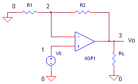
Initially, we test it open-loop by setting R1 = 1 ohm (short) and R2=1e12 (open). For the load, set RL=10k and CL=1pF (effectively no capacitance). To run an AC Analysis, remove the "*" in front of the .AC command and plan an "*" in front of the .TRAN command..

 CIRCUIT INSIGHT   The op amp is driven by AC source VS. There are essentially no feedback resistors here – its running open-loop. Try out the model by running a simulation and plotting the AC magnitude VM(3). Can you see the DC gain = 100k V/V and the first-pole at fp1 = 100 Hz? What is the unity gain frequency? Try changing the Y-Axis to a log scale to get a better view at high frequencies. If your plotting in dB, the unity-gain level is 0 dB.

Now open a new plot window and display the phase VP(3). Does the first pole add -90 deg above the first pole? Check out the phase near 4.8 MHz - do the 2nd and 3rd poles kick in adding another -45 deg for a total of about -135 deg? If so, your ready to close the loop on your device and hit it with a step input in the time domain.

CLOSED-LOOP TEST (TRANSIENT RESPONSE)

Let's close the loop on out amplifier and set it unity gain by setting R1 = 1e12 (open) and R2=1 (short). For the load, set RL=10k and CL=100pF. To run an Transient Analysis, remove the "*" in front of the .TRAN command and plan an "*" in front of the .AC command.

According to the data sheet, the transient response should have a rise time (10% to 90%) of 0.2 us and an overshoot of 10% max.

 CIRCUIT INSIGHT   The op amp is driven by step input of 1 V.  Run a simulation and plot the Transient Response at V(3). What is the rise time and overshoot? It looks like the 10% to 90% rise time is about 0.2 us. Very nice! More good news: you've got some overshoot and ringing - something not easily achievable without the 2nd and 3rd poles. However, the overshoot looks a bit low at only 3%, not quite the 10% shown.

 HANDS-ON DESIGN   Okay, let's do some tweaking. There are two things I usually do. First, lower the 2nd and 3rd pole by 10% or 20%, and second increase ROUT from 100 ohms to 125 or 150 ohms. Try a few tweaks and rerun the simulation. As you lower the poles and raise ROUT, the overshoot should grow. Are you able to raise the overshoot to near 10%? Note that the 10% is a max number and no typical is specified. So it's okay if you don't quite reach 10%.

Your actual circuit will likely behave a bit different due to device variations and some stray capacitance on the PCB. But the simulation has opened your eyes to real world op amp behavior including potential overshoot and ringing.

SIMULATION NOTES

For a description of all op amp models, see Op Amp Models.
This op amp model can be used for many of the op amp circuits available from the Circuit Collection page.

SPICE FILES

Download the file or copy this netlist into a text file with the *.cir extension.

OP_2ND_3RD_POLES.CIR
*
* SIGNAL SOURCE
VS	1	0	AC 1	PWL(0US 0V   0.01US 1V  10US 1V)

* NON INVERTING AMP
R1	0	2	1
R2	2	3	1e12
XOP1	1 2     3       OP_TL062
*
RL	3	0	10k
CL	3	0	1pF

* OP AMP MODEL
*
* Device Pins      In+ In- Vout
.SUBCKT op_tl062    1   2   82
*
* INPUT R
RIN   1   2   1e9
*
*  AMPLIFIER STAGE: GAIN, POLE, SLEW
*   Aol=10000, fu=1000000 Hz
G1   0    10  VALUE = { 1e-2 * V(1,2)  }
R1   10   0   1e6
C1   10   0   1.59159e-9
*
* 2ND POLE 
G2   0 20   10 0  1e-6
R2   20       0     1e6
C2   20       0     3.3e-14
*
* 3RD POLE 
G3   0 30   20 0 1e-6
R3   30       0     1e6
C3   30       0     3.3e-14
*
* OUTPUT STAGE
EBUFFER 80 0  30  0    1
ROUT 80      82        100
.ENDS
*
* ANALYSIS *************************************
*.TRAN 	0.05US  2US
.AC 	DEC 	20 1 100MEG
.PROBE
.END

Top ↑

◄BACK TO OPAMP MODELS

© 2010 eCircuit Center